
‘IPF’ is also known as ‘Raking’ in survey statistics, or ‘Matrix Scaling’ in CS.
Applied & explained

‘Iterative Proportional Fitting’ (a procedure/algorithm re-developed by Deming and Stephan in 1940) is known in many variants and by many names.
In statistics it goes by the name of Iterative Proportional Fitting (IPF), in market research and survey methodology it is often called ‘raking’, while in computer science a similar approach is called ‘matrix scaling’.
What is it, and what can ‘Iterative Proportional Fitting’ do for quant UX research
If we want to be very brief – and let’s day we want 😛 – IPF helps us improve our survey data when we are in a situation when we know that our distribution of certain variables in our sample (survey) does not match the distribution of the population (i.e. reality).
An example makes this easier to understand.
I know from my analytics that my visitors/ app users are 50% male female, and 70% is Dutch and 30% is German. (For this example we assume I have watertight proof that this is the case).
Now my survey results have come back and somehow my survey sample is 60% male and 90% Dutch. This means my sampling or response bias will cause me to overestimate the importance (weight) of Dutch males.
We can solve this by saying we will multiply (weight) the female responses by 50/40 (=1.25) while weighting the male responses by 50/60 (=.83).
However, this can become difficult very quickly as categories increase. Just imagine an e.g. 6 by 3 contingency table..
This is where Iterative Proportional Fitting comes in play. It uses the full contingency table to reestimate the frequencies (through weighting) in our sample so that the marginal distribution of the sample will match the marginal distribution of the population while maintaining relative cell sizes (and this odds ratios) within the table.
For those who like to see this in action, please read on..
I will use an example with real survey data about Belgium from the European Social Survey
(freely available from http://www.europeansocialsurvey.org).
We will look at two variables, one with 6 levels and the second with 3 levels.
On the other hand we have the real populations numbers from the Belgian Labour Force Statistics, where we can see the real proportions with regards to the same variables (https://statbel.fgov.be/)
Proportions in Survey
Proportion in Population
Now through IPF we can use these real proportions from our labour force statistics to calculate weights for our survey data (the ESS data in this example), this helps us correct for our unintended sampling bias, so that our surveys represents the population close to perfectly!
Proportions in survey
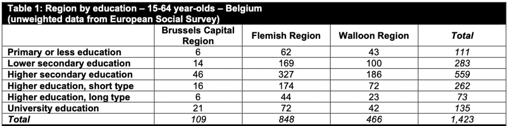
Here we have the 6 (education) by 3 (region) ‘two-way contingency table’ from the European Social Survey mentioned above.

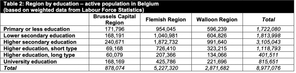
Proportions in population
And here is our table with the same categories but with the real population frequencies, as provided by the Belgian Labour Force Statistics.

We can use IPF to reesimate our survey data table in such a way that it matches the real population statistics with losing the relationships that were present in our survey table.
But before we go ahead with manually applying Iterative Proportional Fitting, we should calculate our local odds ratio’s. This is something that is useful for testing whether our IPF changes do not mess up our original relationships present in our survey data.
Odds Ratio’s Intermezzo
Odds Ratio’s are good for a lot of stuff, but unfortunately they are a bit unfriendly to interpret compared to e.g. probabilities. Below will go into some depth interpreting ans using (local) Odds Ratio’s, so feel free to skip to the IPF part if you are less interested in odds ratio’s.
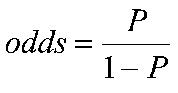
! Remember ‘odds’ =/= probability
Calculating (local) Odds Ratio’s
Local odds ratios (LOR’s) for the region using education levels.
We will consider the variable ‘region’ as our response variable, we will look each of the [(6-1)*(3-1)] = 10 specific local odds ratios instead of just one OR per row
(visualized for ease in table 1).
Local Odds Ratios for all adjacent 2×2’s, with sample’s cell counts in grey.

Firstly, when looking at the relationship between education (taken as x) and region (taken as y), we want to see whether the marginal distribution of region {.08, .60, .33} is identical to the conditional distribution of region. Because if these are identical we are likely looking at independent variables.
Conditional distribution of region (y) given education (x)
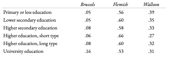
Here we can see the marginal distribution and the conditional distributions are close but not identical. For example, we can spot relatively strong deviation at both extremes of the education variable (i.e. lowest and highest levels) suggesting the two variables are not independent.
Interpreting the odds ratios.
The Local Odds Ratio ‘O11’ (table 1) tells us that the odds of primary/less education versus lower secondary education within the Brussels region (which is .43) is 1.17 times greater than the odds of the same comparison but now in the Flemish region (which is .37) Odds and OR’s smaller than one are generally more easily interpreted when reversed, so the above is more easily understood as follows;
the odds of having secondary education versus primary/less, are 1.17 times greater in the Flemish region (2.73) than in the Brussels region (2.33).
In this manner we can interpret all of the local odds ratios. We can even extend this to OR’s for non-adjacent cells. This way we can for example look at lowest education vs highest in the Brussels region versus that ratio in the Walloon region (This non-adjacent OR is .28.) This can be interpreted (again using the inverse) as the odds of having the lowest education versus the highest in the Walloon region being 3.58 times greater than those odds in the Brussels region.
Without testing we can surmise an interesting overall effect when making sense of the calculated odds ratios’ which is that the higher the level of education the larger the relative odds seems to get with regards to being in/from the Brussels region compared to the other two regions.
Enough with the Odds!
Time for Iterative Proportional Fitting already!
‘Iterative Proportional Fitting’ (IPF) is a weighting procedure used in simple hierarchical loglinear models. This weighting (through IPF) is common in survey data because as surveys are often costly, sampling is used when gathering data (i.e. taking surveys resulting in a subset). Within this subset the frequencies, through chance, selection bias, asymmetric non-response etc, can have different distributions from those of our population. When these population statistics (e.g. the marginal distributions) happen to be known, IPF can help us reestimate the frequencies (through weighting) in our sample so that the marginal distribution of the sample will match the marginal distribution of the population while maintaining relative cell sizes (and this odds ratios) within the table.
Let’s do it
Our aim in the first step is to adjust the cell counts to fit the row marginals, and as a second step we adjust the counts again but now to fit the column marginals. As we have just a two-way table in this example one iteration consists of these two steps. We repeat this (iterate) until the results converge to what we deem sufficient.
The exact steps taken can be seen in detail in this shared google sheet, but I will describe all the steps taken.
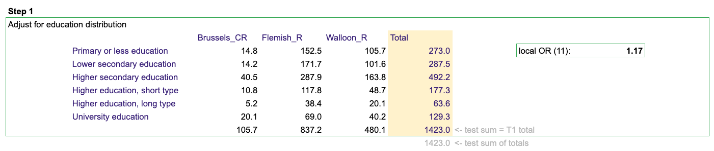
First we adjust the cell counts to fit the row marginals.
In our example this means we take the distribution from table 1 and use this to estimate the cell count using the marginal distribution from table 2
As a second step we adjust the counts again but now to fit the column marginals instead of the row marginals.
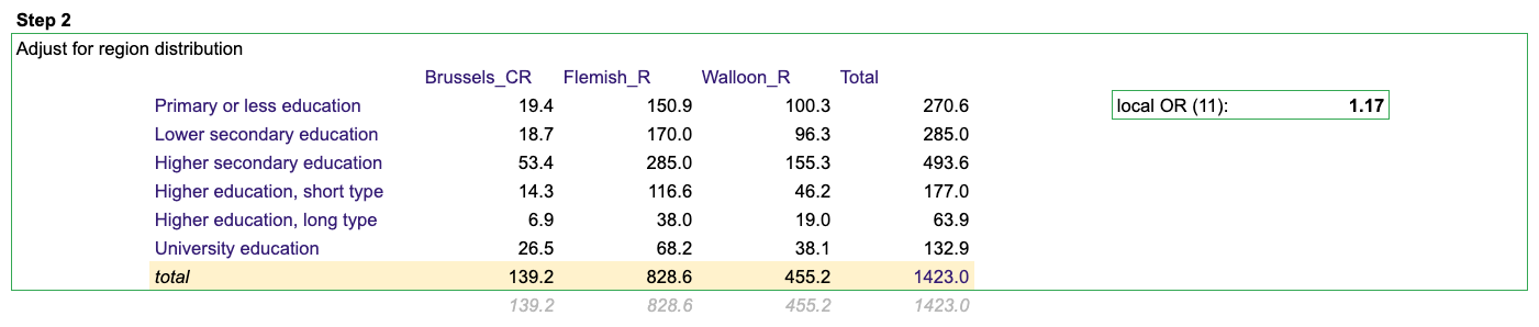
As we have just a two-way table in this example one iteration consists of these two steps. We repeat this (iterate) until the results converge to what we deem sufficient.
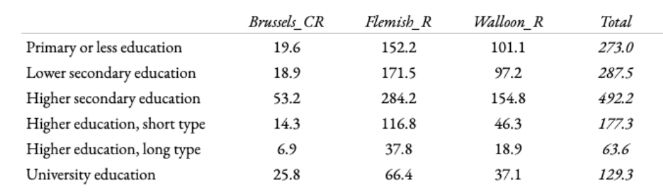
In our example we repeat step 1 (marginal distribution) but now with the adjusted value from step 2.

Here we find our result to be sufficiently converged and stop, but it is possible to continue further in order to further diminish the difference until they are even smaller.
If have made an open version of the excel sheet, so if desired it is possible to see the exact calculations per step here.
The re-estimated table using IPF (Deming-Stephan Adjustment) as described above.
Finally, by re-calculating the odds ratios using the new values we can verify the original relationships are still the same after our procedure of Iterative proportional fitting.